

PXIe System - High-Performance Modular Test Platform
PXIe high-performance measurement system is based on PXle Bus and DSP board structure by the combination of different data acquisition card and output interface card, can realize largescale-channel distributed data acquisition and centralized processing, one-way transmission speed is up to 250 MB/s, ensure the multichannel parallel acquisition and real time closed-loop control.
Up to 16 output channels for single unit, control 16 shakers simultaneously.
High precision: 24-bit AD/DA, 32-bit 450 MHz DSP processing, 135dB dynamic range,
Powerful transmission and processing capacity: Based on PXIe bus and embedded real-time operating system, the transmission rate can up to 250 MB/s by point-to-point one-way transmission, high real-time control.
Output channel is full isolation design, Minimize external distractions, Improve the signal-tonoise ratio of the test system.
Low power consumption: adopt DSP floating ground design, higher energy efficiency, lower heat dissipation.
Extension: 21EX single mainframe input up to 168 channels (DAQ), 10EX single mainframe input up to 80 channels (DAQ)
Powerful Data acquisition software with a wide variety of analysis modules.
Measured: acceleration, microphone, tachometer/Count, CAN module, digital signal I/O (DI/O), RS485, strain gage, displacement, velocity, force, pressure, temperature/Humidity, current Signal(4-20mA), other Bridge Sensor, other sensor (IEPE or Charge).
Signal source: sine, sine sweep frequency, white noise, blasting random, forming random, forming random, pseudo-random, whistle, triangular wave, rectangular wave, DC, pulse and so on a total of 12 signal types.
| Model | 10EX | 21EX |
|---|---|---|
| Slots | 10 | 21 |
| Output channel | Max. 24ch | Max. 24ch |
| Input channel | Max. 80ch | Max. 168ch |
| Abort port | ✓ | ✓ |
| Input mode AC |
✓ | ✓ |
| DC | ✓ | ✓ |
| ICP (ICP Comm Indicator: Different connection status of the ICP sensor) |
✓ | ✓ |
| Charge (Built-in charge amplifier) |
✓ | ✓ |
| TEDS | ✓ | ✓ |
| Digital I/O | Configurable digital I/O card, 8-bit input, 8-bit output | |
| Bus | PXIe bus | |
| Embedded Computer | Real time operating system (Dual-core, 2.2GHz CPU, 16GB RAM) | |
| Built-in hard disk | 1 TB NVMe | |
| DSP | 450 MHz 的 32-bit floating DSP | |
| Size | 222*177*271 mm | 445*177*271 mm |
| Weight | about 9.5 kg | about 18 kg |
| Power | Voltage range (100~240)VAC, Frequency range (50~60)Hz | |
| Rated power 200 W | Rated power 400 W | |
| Main chassis interface | Gigabit Ethernet interface | |
| Software operating environment | Microsoft Windows XP/7/8/10/11 | |
| Data acquisition function | Basic Platform Software, Spectrum Analysis Module, FRF Analysis Module, Octave Analysis Module, SRS Analysis Module, Shock Pulse Detection Module, Cepstrum Analysis Module, Correlation Analysis Module, Probabilistic and Statistical Analysis Module, Calculus Module, Digital Filter Module, Damping Ratio Computation Module, Modal Analysis Module, Rain-flow Counting Method Module, Sound Pressure Module, Air-conditioner Test and Analysis Module, Sweepfrequency Analysis Module, Audio Playing Module, Alarm Module, Timed Text File Output Module, Multisensor Calibration Module, Device Status Diagram | |
| CE certification | |
|---|---|
| Safety standard | Satisfy EN 61010-1 |
| EMC | Satisfy EN 61326-1 Class A emissions; Basic immunity, EN 55011: Group 1, Class A emissions |
| Working environment | Temperature Range (0~50) Humidity Range (20~90)%RH |
| Antivibration Performance | Working condition: 5~500 Hz, 0.3 grms Non-working condition: 5~500 Hz, 2.4 grms (According to IEC 68-2-64) |
| Shock Resistance | Working condition: Half-sine 30 g, 11 ms (According to IEC 68-2-27) |
| Input channel specification | |||
|---|---|---|---|
| Model | 10EX | 21EX | |
| Voltage/Charge Acquisition Card | Input channel | 8 ~ 80 | 8 ~ 168 |
| Channel No. (one-card) | 8 | ||
| Measured | Acceleration (IEPE), Microphone (IEPE), Tachometer/Count, CAN Module, Digital signal I/O (DI/O), RS485, Displacement, Velocity, Force, Pressure, Temperature/Humidity, Current Signal (4–20mA), All Sensor (voltage output) | ||
| Output Interface | SMB, BNC Connector | ||
| A/D Conversion | 24-bit | ||
| Dynamic Range | 135 dB | ||
| SNR | > 100 dB | ||
| Input Range | ±0.1 Vpk, ±1.0 Vpk, ±10 Vpk | ||
| Input Protection | ±36 Vpk no damaging | ||
| Accuracy Amplitude | <0.1%(@1V, 1 kHz) | ||
| Input Impedance | 200 kΩ | ||
| Channel Matching | Amplitude Ratio: ±0.1 dB, Phase Differences: ±1.0° (1 Hz~20 kHz) | ||
| Channel Interference | <100 dB@1 kHz | ||
| Harmonic Distortion | <-100 dB@1 kHz | ||
| Anti-alias Filter | Analog and digital anti-aliasing low pass filter | ||
| Strain Acquisition Card | Channel No. (one-card) | 8 | |
| Measured | Strain Gage, Other Bridge Sensor | ||
| Input Interface | LEMO 0B | ||
| A/D conversion | 24-bit | ||
| Built-in Bridge | full bridge, half bridge, 1/4 bridge (120 ohms) | ||
| Strain Gauge Resistance Value | <10k ohms | ||
| Bridge Voltage | 0V–20V (adjustable) | ||
| Bridge Compression Accuracy | <0.1% | ||
| Self-balancing Range | ±20000με | ||
| Voltage Range | ±10V, ±1V, ±100mV, ±10mV | ||
| Voltage Indication Error | <0.3% | ||
| Strain Range | ±1000με, ±10000με, ±100000με | ||
| Strain Indication Error | ±(0.3%red±3με) (preheat for 1 hour) | ||
| Input Impedance | 10 MΩ+10 MΩ | ||

Modal Analysis
Geometric Modeling
Draw geometric elements: Draw points, lines, triangles, circles, planes, balls.
Draw advanced geometry elements: Draw stretches, move, copy, rotate, scale.
Import external 3D geometry models: STL and other common formats.
Modal Parameter Identification
Navigational modal parameter identification: Function selection, order estimation, parameter estimation, function synthesis and synthesis display.
Order estimation: Modal segmentation, modal peak function, multimodal peak function, complex modal indication function.
Parameter estimation: Identification of modal parameters such as natural frequency and damping ratio.
Function synthesis: Generate a comprehensive frequency response function.
Comprehensive display: Multi-view visual display of the measured frequency response and comprehensive frequency response in the amplitude-frequency characteristics of the consistency.
Mode Simulation
Time domain ODS: The driving data comes from the time history data, displays the real time history movement of the structure, and 3D color simulation animation.
Frequency domain ODS: Drive data from the frequency domain function, display structure movement under sine excitation, 3D color simulation animation.
Modal shape: Drive data from mode mode, 3D color simulation animation. Animation simulation control: Motion control, attempt control, display control, recording video.
MAC modal confidence criteria
MAC modal confidence criteria: For comparison of modal similarity, the modal confidence criteria table can be displayed as color graphs and three-dimensional bar graphs.
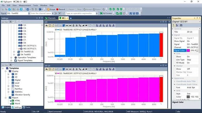
Octave Analysis
Octave
Bandwidth indicator values: 1/1, 1/3, 1/6, 1/12, 1/24.
Start frequency, End frequency: configurable.
Sampling frequency: Automatically adjusted according to the set end frequency, up to 204.8kHz.
Frequency weight: linear weight, A/B/C/D weight.
Average
Average mode: linear average, exponential average.
Time constant: 35ms (pulse), 65ms, 125ms (fast), 250ms, 500ms, 1s(slow), 2s, 5s, 10s, 20s.
Hold: Disable, maximum, minimum.
Transition signal
Rejection: Optional.
Detection
Detection type: A&L, B&L, C&L, D&L.
Total Value Frame size: 256 to 4096 Optional.
Step time: can be set.
Display window
Window type: 2D diagram, 3D diagram(waterfall/color diagram), trajectory diagram, polar coordinate diagram, long waveform diagram, large text diagram, channel level indicator diagram, picture pane, etc.
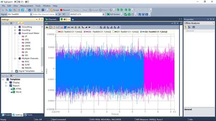
Acoustic Analysis
Acoustic analysis is a comprehensive and versatile solution for sound signal processing, noise evaluation, and sound intensity testing. Here's a breakdown of its key features and capabilities:
1. Data Processing & Windowing
Manual Data Selection: Users can manually define the length of each data segment for analysis.
Processing Methods:
Instantaneous analysis (real-time snapshot)
Linear averaging (equal weight over time)
Exponential averaging (weighted toward recent data)
Maximum value retention (peak detection)
Windowing Functions (to reduce spectral leakage):
Rectangular window
Hanning window
Hamming window
(Possibly others like Blackman, Flat-top, etc.)
2. Spectral Analysis Options
Narrowband Spectrum (high-resolution FFT)
Octave Band Analysis (for standardized frequency bands):
1/1 Octave (broadband)
1/3 Octave (common in noise measurements)
1/12 Octave (higher resolution)
1/24 Octave (very fine resolution)
Frequency Weighting Filters (mimicking human hearing):
L (Linear, no weighting)
A-weighting (low-level sounds, common in environmental noise)
B-weighting (mid-level sounds, less common)
C-weighting (high-level sounds, industrial noise)
D-weighting (aircraft noise)
3. Noise & Sound Quality Evaluation
Noise Metrics (e.g., Leq, Lmax, Lmin, SEL, etc.)
Psychoacoustic Indicators:
Loudness (perceived intensity, e.g., in sones or phons)
Sharpness (high-frequency content)
(Possibly others like roughness, fluctuation strength, tonality)
Real-time & Offline Processing (flexible for different use cases)
4. Sound Intensity Testing (20Hz–20kHz)
Sound Pressure-Sound Pressure (p-p) Probe Method:
Measures active sound intensity (vector quantity) for sound source localization.
3D Visualization:
Tables (numeric data)
Contour Maps (2D intensity distribution)
3D Distribution Maps (spatial sound field)
Sound Source Localization:
2D/3D Sound Intensity Cloud Maps (color-coded intensity grids)
5. Microphone Calibration & Management
Multi-Channel Calibration: Fast calibration for array setups.
Microphone Database:
Stores calibration data for each microphone.
Allows easy retrieval and management for consistent measurements.